


Lace is a probabilistic cross-categorization engine written in rust with an optional interface to python. Unlike traditional machine learning methods, which learn some function mapping inputs to outputs, Lace learns a joint probability distribution over your dataset, which enables users to...
- predict or compute likelihoods of any number of features conditioned on any number of other features
- identify, quantify, and attribute uncertainty from variance in the data, epistemic uncertainty in the model, and missing features
- determine which variables are predictive of which others
- determine which records/rows are similar to which others on the whole or given a specific context
- simulate and manipulate synthetic data
- work natively with missing data and make inferences about missingness (missing not-at-random)
- work with continuous and categorical data natively, without transformation
- identify anomalies, errors, and inconsistencies within the data
- edit, backfill, and append data without retraining
and more, all in one place, without any explicit model building.
import pandas as pd
import lace
# Create an engine from a dataframe
df = pd.read_csv("animals.csv", index_col=0)
engine = lace.Engine.from_df(df)
# Fit a model to the dataframe over 5000 steps of the fitting procedure
engine.update(5000)
# Show the statistical structure of the data -- which features are likely
# dependent (predictive) on each other
engine.clustermap("depprob", zmin=0, zmax=1)
The Problem
The goal of lace is to fill some of the massive chasm between standard machine learning (ML) methods like deep learning and random forests, and statistical methods like probabilistic programming languages. We wanted to develop a machine that allows users to experience the joy of discovery, and indeed optimizes for it.
Short version
Standard, optimization-based ML methods don't help you learn about your data. Probabilistic programming tools assume you already have learned a lot about your data. Neither approach is optimized for what we think is the most important part of data science: the science part: asking and answering questions.
Long version
Standard ML methods are easy to use. You can throw data into a random forest and start predicting with little thought. These methods attempt to learn a function f(x) -> y that maps inputs x, to outputs y. This ease-of-use comes at a cost. Generally f(x) does not reflect the reality of the process that generated your data, but was instead chosen by whoever developed the approach to be sufficiently expressive to better achieve the optimization goal. This renders most standard ML completely uninterpretable and unable to yield sensible uncertainty estimate.
On the other extreme you have probabilistic tools like probabilistic programming languages (PPLs). A user specifies a model to a PPL in terms of a hierarchy of probability distributions with parameters θ. The PPL then uses a procedure (normally Markov Chain Monte Carlo) to learn about the posterior distribution of the parameters given the data p(θ|x). PPLs are all about interpretability and uncertainty quantification, but they place a number of pretty steep requirements on the user. PPL users must specify the model themselves from scratch, meaning they must know (or at least guess) the model. PPL users must also know how to specify such a model in a way that is compatible with the underlying inference procedure.
Example use cases
- Combine data sources and understand how they interact. For example, we may wish to predict cognitive decline from demographics, survey or task performance, EKG data, and other clinical data. Combined, this data would typically be very sparse (most patients will not have all fields filled in), and it is difficult to know how to explicitly model the interaction of these data layers. In Lace, we would just concatenate the layers and run them through.
- Understanding the amount and causes of uncertainty over time. For example, a farmer may wish to understand the likelihood of achieving a specific yield over the growing season. As the season progresses, new weather data can be added to the prediction in the form of conditions. Uncertainty can be visualized as variance in the prediction, disagreement between posterior samples, or multi-modality in the predictive distribution (see this blog post for more information on uncertainty)
- Data quality control. Use
surprisalto find anomalous data in the table and use-logpto identify anomalies before they enter the table. Because Lace creates a model of the data, we can also contrive methods to find data that are inconsistent with that model, which we have used to good effect in error finding.
Who should not use Lace
There are a number of use cases for which Lace is not suited
- Non-tabular data such as images and text
- Highly optimizing specific predictions
- Lace would rather over-generalize than over fit.
Quick start
Installation
Lace requires rust.
To install the CLI:
$ cargo install --locked lace-cli
To install pylace
$ pip install pylace
Examples
Lace comes with two pre-fit example data sets: Satellites and Animals.
>>> from lace.examples import Satellites
>>> engine = Satellites()
# Predict the class of orbit given the satellite has a 75-minute
# orbital period and that it has a missing value of geosynchronous
# orbit longitude, and return epistemic uncertainty via Jensen-
# Shannon divergence.
>>> engine.predict(
... 'Class_of_Orbit',
... given={
... 'Period_minutes': 75.0,
... 'longitude_radians_of_geo': None,
... },
... )
('LEO', 0.023981898950561048)
# Find the top 10 most surprising (anomalous) orbital periods in
# the table
>>> engine.surprisal('Period_minutes') \
... .sort('surprisal', reverse=True) \
... .head(10)
shape: (10, 3)
┌─────────────────────────────────────┬────────────────┬───────────┐
│ index ┆ Period_minutes ┆ surprisal │
│ --- ┆ --- ┆ --- │
│ str ┆ f64 ┆ f64 │
╞═════════════════════════════════════╪════════════════╪═══════════╡
│ Wind (International Solar-Terres... ┆ 19700.45 ┆ 11.019368 │
│ Integral (INTErnational Gamma-Ra... ┆ 4032.86 ┆ 9.556746 │
│ Chandra X-Ray Observatory (CXO) ┆ 3808.92 ┆ 9.477986 │
│ Tango (part of Cluster quartet, ... ┆ 3442.0 ┆ 9.346999 │
│ ... ┆ ... ┆ ... │
│ Salsa (part of Cluster quartet, ... ┆ 3418.2 ┆ 9.338377 │
│ XMM Newton (High Throughput X-ra... ┆ 2872.15 ┆ 9.13493 │
│ Geotail (Geomagnetic Tail Labora... ┆ 2474.83 ┆ 8.981458 │
│ Interstellar Boundary EXplorer (... ┆ 0.22 ┆ 8.884579 │
└─────────────────────────────────────┴────────────────┴───────────┘
And similarly in rust:
use lace::prelude::*;
use lace::examples::Example;
fn main() {
// In rust, you can create an Engine or and Oracle. The Oracle is an
// immutable version of an Engine; it has the same inference functions as
// the Engine, but you cannot train or edit data.
let mut engine = Example::Satellites.engine().unwrap();
// Predict the class of orbit given the satellite has a 75-minute
// orbital period and that it has a missing value of geosynchronous
// orbit longitude, and return epistemic uncertainty via Jensen-
// Shannon divergence.
engine.predict(
"Class_of_Orbit",
&Given::Conditions(vec![
("Period_minutes", Datum:Continuous(75.0)),
("Longitude_of_radians_geo", Datum::Missing),
]),
Some(PredictUncertaintyType::JsDivergence),
None,
)
}Fitting a model
To fit a model to your own data you can use the CLI
$ lace run --csv my-data.csv -n 1000 my-data.lace
...or initialize an engine from a file or dataframe.
>>> import pandas as pd # Lace supports polars as well
>>> from lace import Engine
>>> engine = Engine.from_df(pd.read_csv("my-data.csv", index_col=0))
>>> engine.update(1_000)
>>> engine.save("my-data.lace")
You can monitor the progress of the training using diagnostic plots
>>> from lace.plot import diagnostics
>>> diagnostics(engine)
License
Lace is licensed under the MIT licenses as of v0.9.0.
Installation
Installation requires rust, which you can get here.
CLI
The lace CLI is installed with rust via the command
$ cargo install --locked lace-cli
Rust crate
To use the lace crate in a rust project add the following line under the
dependencies block in your Cargo.toml:
lace = "<version>"
Python
The python library can be installed with pip
pip install
The lace workflow
The typical workflow consists of two or three steps:
Step 1 is optional in many cases as Lace usually does a good job of inferring the types of your data. The condensed workflow looks like this.
import pandas as pd
import lace
df = pd.read_csv("mydata.csv", index_col=0)
# 1. Create a codebook (optional)
codebook = lace.Codebook.from_df(df)
# 2. Initialize a new Engine from the prior. If no codebook is provided, a
# default will be generated
engine = lace.Engine.from_df(df, codebook=codebook)
# 3. Run inference
engine.run(5000)
use polars::prelude::{SerReader, CsvReader};
use lace::prelude::*;
let df = CsvReader::from_path("mydata.csv")
.unwrap()
.has_header(true)
.finish()
.unwrap();
// 1. Create a codebook (optional)
let codebook = Codebook::from_df(&df, None, None, False).unwrap();
// 2. Build an engine
let mut engine = EngineBuilder::new(DataSource::Polars(df))
.with_codebook(codebook)
.build()
.unwrap();
// 3. Run inference
// Use `run` to fit with the default transition set and update handlers; use
// `update` for more control.
engine.run(5_000);You can also use the CLI to create codebooks and run inference. Creating a default YAML codebook with the CLI, and then manually editing is good way to fine tune models.
$ lace codebook --csv mydata.csv codebook.yaml
$ lace run --csv data.csv --codebook codebook.yaml -n 5000 metadata.lace
Create and edit a codebook
The codebook contains information about your data such as the row and column names, the types of data in each column, how those data should be modeled, and all the prior distributions on various parameters.
The default codebook
In the lace CLI, you have the ability to initialize and run a model without specifying a codebook.
$ lace run --csv data -n 5000 metadata.lace
Behind the scenes, lace creates a default codebook by inferring the types of your columns and creating a very broad (but not quite broad enough to satisfy the frequentists) hyper prior, which is a prior on the prior.
We can also create the default codebook in code.
import polars as pl
from lace import Codebook
from lace.examples import ExamplePaths
# Here we get the path to an example csv file, but you can use any file that
# can be read into a polars or pandas dataframe
path = ExamplePaths("satellites").data
df = pl.read_csv(path)
# Infer the default codebook for df
codebook = Codebook.from_df("satellites", df)
use polars::prelude::{CsvReadOptions, SerReader};
use lace::codebook::Codebook;
use lace::examples::Example;
// Load an example file
let paths = Example::Satellites.paths().unwrap();
let df = CsvReadOptions::default()
.with_has_header(true)
.try_into_reader_with_file_path(Some(paths.data))
.unwrap()
.finish()
.unwrap();
// Create the default codebook
let codebook = Codebook::from_df(&df, None, None, None, false).unwrap();Creating a template codebook
Lace is happy to generate a default codebook for you when you initialize a model. You can create and save the default codebook to a file using the CLI. To create a codebook from a CSV file:
$ lace codebook --csv data.csv codebook.yaml
Note that if you love quotes and brackets, and hate being able to comment, you can use json for
the codebook. Just give the output of codebook a .json extension.
$ lace codebook --csv data.csv codebook.json
If you use a data format with a schema, such as Parquet or IPC (Apache Arrow v2), you make Lace's work a bit easier.
$ lace codebook --ipc data.arrow codebook.yaml
If you want to make changes to the codebook -- the most common of which are editing the Dirichlet process prior, specifying whether certain columns are missing not-at-random, adjusting the prior distributions and disabling hyper priors -- you just open it up in your text editor and get to work.
For example, let's say we wanted to make a column of the satellites data set missing not-at-random, we first create the template codebook,
$ lace codebook --csv satellites.csv codebook-sats.yaml
open it up in a text editor and find the column of interest
- name: longitude_radians_of_geo
coltype: !Continuous
hyper:
pr_m:
mu: 0.21544247097911842
sigma: 1.570659039531299
pr_k:
shape: 1.0
rate: 1.0
pr_v:
shape: 6.066108090103747
scale: 6.066108090103747
pr_s2:
shape: 6.066108090103747
scale: 2.4669698184613824
prior: null
notes: null
missing_not_at_random: false
{
"name": "longitude_radians_of_geo",
"coltype": {
"Continuous": {
"hyper": {
"pr_m": {
"mu": 0.21544247097911842,
"sigma": 1.570659039531299
},
"pr_k": {
"shape": 1.0,
"rate": 1.0
},
"pr_v": {
"shape": 6.066108090103747,
"scale": 6.066108090103747
},
"pr_s2": {
"shape": 6.066108090103747,
"scale": 2.4669698184613824
}
},
"prior": null
}
},
"notes": null,
"missing_not_at_random": false
}
and change the column metadata to something like this:
- name: longitude_radians_of_geo
coltype: !Continuous
hyper:
pr_m:
mu: 0.21544247097911842
sigma: 1.570659039531299
pr_k:
shape: 1.0
rate: 1.0
pr_v:
shape: 6.066108090103747
scale: 6.066108090103747
pr_s2:
shape: 6.066108090103747
scale: 2.4669698184613824
prior: null
notes: "This value is only defined for GEO satellites"
missing_not_at_random: true
{
"name": "longitude_radians_of_geo",
"coltype": {
"Continuous": {
"hyper": {
"pr_m": {
"mu": 0.21544247097911842,
"sigma": 1.570659039531299
},
"pr_k": {
"shape": 1.0,
"rate": 1.0
},
"pr_v": {
"shape": 6.066108090103747,
"scale": 6.066108090103747
},
"pr_s2": {
"shape": 6.066108090103747,
"scale": 2.4669698184613824
}
},
"prior": null
}
},
"notes": null,
"missing_not_at_random": true
}
Sometimes, we have a bit of knowledge that we can transfer to lace in the form of a more-specific prior distribution. To set the prior we remove the hyper prior and set the prior. Note that doing this disabled prior parameter inference.
- name: longitude_radians_of_geo
coltype: !Continuous
hyper: null
prior:
m: 0.0
k: 1.0
v: 1.0
s2: 3.0
notes: "This value is only defined for GEO satellites"
missing_not_at_random: true
{
"name": "longitude_radians_of_geo",
"coltype": {
"Continuous": {
"hyper": null,
"prior": {
"m": 0.0,
"k": 1.0,
"v": 1.0,
"s2": 3.0
}
}
},
"notes": null,
"missing_not_at_random": true
}
For a complete list of codebook fields, see the reference.
Run/train/fit a model
Lace is a Bayesian tool so we do posterior sampling via Markov chain Monte Carlo (MCMC). A typical machine learning model will use some sort of optimization method to find one model that fits best; the objective for fitting is different in Lace.
In Lace we use a number of states (or samples), each running MCMC independently to characterize the posterior distribution of the model parameters given the data. Posterior sampling isn't meant to maximize the fit to a dataset, it is meant to help understand the conditions that created the data.
When you fit to your data in Lace, you have options to run a set number of
states for a set number of iterations (limited by a timeout). Each state is a
posterior sample. More states is better, but the run time of everything
increases linearly with the number of states; not just the fit, but also the
OracleT operations like logp and simulate. As a rule of thumb, 32 is a
good default number of states. But if you find your states tend to strongly
disagree on things, it is probably a good idea to add more states to fill in
the gaps.
As for number of iterations, you will want to monitor your convergence plots. There is no benefit of early stopping like there is with neural networks. MCMC will usually only do better the longer you run it and Lace is not likely to overfit like a deep network.

The above figure shows the MCMC algorithm partitioning a dataset into views and categories.
A (potentially useless) analogy comparing MCMC to optimization
At the risk of creating more confusion than we resolve, let us make an analogy to mountaineering. You have two mountaineers: a gradient ascent (GA) mountaineer and an MCMC mountaineer. You place each mountaineer at a random point in the Himalayas and say "go". GA's goal is to find the peak of Everest. Its algorithm for doing so is simply always to go up and never to go down. GA is guaranteed to find a peak, but unless it is very lucky in its starting position, it is unlikely ever to summit Everest.
MCMC has a different goal: to map the mountain range (posterior distribution). It does this by always going up, but sometimes going down if it doesn't end up too low. The longer MCMC explores, the better understanding it gains about the Himalayas: an understanding which likely includes a good idea of the position of the peak of Everest.
While GA achieves its goal quickly, it does so at the cost of understanding the terrain, which in our analogy represents the information within our data.
In Lace we place a troop of mountaineers in the mountain range of our posterior distribution. We call individuals mountaineers states or samples, or chains. Our hope is that our mountaineers can sufficiently map the information in our data. Of course the ability of the mountaineers to build this map depends on the size of the space (which is related to the size of the data) and the complexity of the space (the complexity of the underlying process)
In general the posterior of a Dirichlet process mixture is indeed much like the Himalayas in that there are many, many peaks (modes), which makes the mountaineer's job difficult. Certain MCMC kernels do better in certain circumstances, and employing a variety of kernels leads to better result.
Our MCMC Kernels
The vast majority of the fitting runtime is updating the row-category assignment and the column-view assignment. Other updates such as feature components parameters, CRP parameters, and prior parameters, take an (relatively) insignificant amount of time. Here we discuss the MCMC kernels responsible for the vast majority of work in Lace: the row and column reassignment kernels:
Row kernels
- slice: Proposes reassignment for each row to an instantiated category or
one of many new, empty categories. Slice is good for small tweaks in the
assignment, and it is very fast. When there are a lot of rows,
slicecan have difficulty creating new categories. - gibbs: Proposes reassignment of each row sequentially. Generally makes
larger moves than
slice. Because it is sequential, and accesses data in random order,gibbsis very slow. - sams: Proposes mergers and splits of categories. Only considers the rows in
one or two categories. Proposes large moves, but cannot make the fine
tweaks that
sliceandgibbscan. Since it proposes big moves, its proposals are often rejected as the run progresses and the state is already fitting fairly well.
Column kernels
The column kernels are generally adapted from the row kernels with some caveats.
- slice: Same as the row kernel, but over columns.
- gibbs: The same structurally as the row kernel, but uses random seed control to implement parallelism.
Gibbs is a good choice if the number of columns is high and mixing is a concern.
Fitting models in code
Though the CLI is a convenient way to fit models and generate metadata files outside of python or rust, you may often times find yourself wanting to fit in code. Lace gives you a number of options in both rust and python.
Rust
We first initialize a new Engine:
use rand::SeedableRng;
use rand_xoshiro::Xoshiro256Plus;
use polars::prelude::{CsvReadOptions, SerReader};
use lace::prelude::*;
use lace::examples::Example;
// Load an example file
let paths = Example::Satellites.paths().unwrap();
let df = CsvReadOptions::default()
.with_has_header(true)
.try_into_reader_with_file_path(Some(paths.data))
.unwrap()
.finish()
.unwrap();
// Create the default codebook
let codebook = Codebook::from_df(&df, None, None, None, false).unwrap();
// Build an rng
let rng = Xoshiro256Plus::from_os_rng();
// This initializes 32 states from the prior
let mut engine = Engine::new(
32,
codebook,
DataSource::Polars(df),
0,
rng,
).unwrap();Now we have two options for fitting. We can use the Engine::run method, which
uses a default set of transition operations that prioritizes speed.
engine.run(1_000);We can also tell lace exactly which transitions to run.
// Run for 1000 iterations. Use the Gibbs column reassignment kernel, and
// alternate between the merge-split (Sams) and slice row kernels
let run_config = EngineUpdateConfig::new()
.n_iters(100)
.transitions(vec![
StateTransition::ColumnAssignment(ColAssignAlg::Gibbs),
StateTransition::StatePriorProcessParams,
StateTransition::RowAssignment(RowAssignAlg::Sams),
StateTransition::ComponentParams,
StateTransition::RowAssignment(RowAssignAlg::Slice),
StateTransition::ComponentParams,
StateTransition::ViewPriorProcessParams,
StateTransition::FeaturePriors,
]);
engine.update(run_config.clone(), ()).unwrap();Note the second argument to engine.update. This is the update handler, which
allows users to do things like attach progress bars, handle Ctrl+C, and collect
additional diagnostic information. There are a number a built-ins for common use
case, but you can implement UpdateHandler for your own types if you need extra
capabilities. () is the null update handler.
If we wanted a simple progressbar
use lace::prelude::update_handler::ProgressBar;
engine.update(run_config.clone(), ProgressBar::new()).unwrap();Or if we wanted a progress bar and a Ctrl+C handler, we can use a tuple of UpdateHandlers.
use lace::prelude::update_handler::CtrlC;
engine.update(
run_config,
(ProgressBar::new(), CtrlC::new())
).unwrap();Python
Let's load an Engine from an example and run it with the default transitions
for 1000 iterations.
from lace.examples import Satellites
engine = Satellites()
engine.update(100)
As in rust, we can control which transitions are run. Let's just update the row assignments a bunch of times.
from lace import RowKernel, StateTransition
engine.update(
500,
timeout=10, # each state can run for at most 10 seconds
checkpoint=250, # save progress every 250 iterations
save_path="mydata.lace",
transitions=[
StateTransition.row_assignment(RowKernel.slice()),
StateTransition.view_prior_process_params(),
],
)
Convergence
When training a neural network, we monitor for convergence in the error or loss. When, say, we see diminishing returns in our loss function with each epoch, or we see overfitting in the validation set, it is time to stop. Convergence in MCMC is a bit different. We say our Markov Chain has converged when it has settled into a situation in which it is producing draws from the posterior distribution. In the beginning state of the chain, it is rapidly moving away from the low probability area in which it was initialized and into the higher probability areas more representative of the posterior.
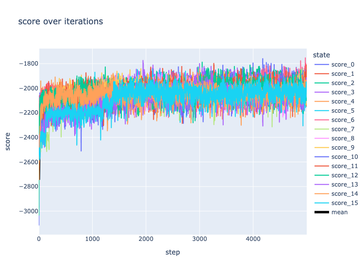
To monitor convergence, we observe the score (which is proportional to the likelihood) over time. If the score stops increasing and begins to oscillate, one of two things has happened: we have settled into the posterior distribution, or the Markov Chain has gotten stuck on an island of high likelihood. When a model is identifiable (meaning that each unique parameter set creates a unique model) the posterior distribution is unimodal, which means there is only one peak, which is easily mapped.
Above. Score by MCMC kernel step in the Animals dataset. Colored lines represent the scores of parallel Markov Chains; the black line is their mean.
Above. Score by MCMC kernel step in the Satellites dataset. Colored lines represent the scores of parallel Markov Chains; the Black line is their mean. Note that some of the Markov Chains experience sporadic jumps upward. This is the MCMC kernel hopping to a higher-probability mode.
A Bayesian modeler must make a compromises between expressiveness, interpretability, and identifiablity. A modeler may transform variables to create a more well-behaved posterior at the cost of the model being less interpretable. The modeler may also achieve identifiablity by reducing the complexity of the model at the cost of failing to capture certain phenomena.
To be general, a model must be expressive, and to be safe, a model must be interpretable. We have chosen to favor general applicability and interpretability over identifiablity. We fight against multimodality in three ways: deploying MCMC algorithms that are better at hopping between modes, by running many Markov Chains in parallel, and by being interpretable.
There are many metrics for convergence but none of the them are practically useful for models of this complexity. Instead we encourage users to monitor convergence via the score and by smell-testing the model. If your model is failing to pick up obvious dependencies, or is missing out on obvious intuitions, you should run it more.
Conduct an analysis
You've made a codebook, you've fit a model, now you're ready to do learn.
Let's use the built-in examples to walk through some key concepts. The
Animals example isn't the biggest, or most complex, and that's exactly why
it's so great. People have acquired a ton of intuition about animals like how
and why you might categorize animals into a taxonomy, and why animals have
certain features and what that might tell us about other features of animals.
This means, that we can see if lace recovers our intuition.
from lace import examples
# if this is your first time using the example, lace must
# build the metadata
animals = examples.Animals()
use lace::examples::Example;
use lace::prelude::*;
// You can create an Engine or an Oracle. An Oracle is
// basically an immutable Engine. You cannot add/edit data or
// extend runs (update).
let animals = Example::Animals.engine().unwrap();Statistical structure
Usually, the first question we want to ask of a new dataset is "What questions can I answer?" This is a question about statistical dependence. Which features of our dataset share statistical dependence with which others? This is closely linked with the question "which things can I predict given which other things?"
In python, we can generate a plotly heatmap of dependence probability.
animals.clustermap(
'depprob',
color_continuous_scale='greys',
zmin=0,
zmax=1
).figure.show()
In rust, we ask about dependence probabilities between individual pairs of features
let depprob_flippers = animals.depprob(
"swims",
"flippers",
).unwrap();Prediction
Now that we know which columns are predictive of each other, let's do some predicting. We'll predict whether an animal swims. Just an animals. Not an animals with flippers, or a tail. Any animal.
animals.predict("swims")
animals.predict(
"swims",
&Given::<usize>::Nothing,
true,
None,
);Which outputs
(0, 0.04384630488890182)
The first number is the prediction. Lace predicts that an animal does not swims (because most of the animals in the dataset do not swim). The second number is the uncertainty. Uncertainty is a number between 0 and 1 representing the disagreement between states. Uncertainty is 0 if all the states completely agree on how to model the prediction, and is 1 if all the states completely disagree. Note that uncertainty is not tied to variance.
The uncertainty of this prediction is very low.
We can add conditions. Let's predict whether an animal swims given that it has flippers.
animals.predict("swims", given={'flippers': 1})
animals.predict(
"swims",
&Given::Conditions(vec![
("flippers", Datum::Categorical(lace::Category::UInt(1)))
]),
true,
None,
);Output:
(1, 0.09588592928237495)
The uncertainty is a little higher, but still quite low.
Let's add some more conditions that are indicative of a swimming animal and see how that effects the uncertainty.
animals.predict("swims", given={'flippers': 1, 'water': 1})
animals.predict(
"swims",
&Given::Conditions(vec![
("flippers", Datum::Categorical(lace::Category::UInt(1))),
("water", Datum::Categorical(lace::Category::UInt(1))),
]),
true,
None,
);Output:
(1, 0.06761776764962134)
The uncertainty is a bit lower now that we've added swim-consistent evidence.
How about we try to mess with Lace? Let's try to confuse it by asking it to predict whether an animal with flippers that does not go in the water swims.
animals.predict("swims", given={'flippers': 1, 'water': 0})
animals.predict(
"swims",
&Given::Conditions(vec![
("flippers", Datum::Categorical(lace::Category::UInt(1))),
("water", Datum::Categorical(lace::Category::UInt(0))),
]),
true,
None,
);Output:
(0, 0.36077426258767503)
The uncertainty is really high! We've successfully confused lace.
Evaluating likelihoods
Let's compute the likelihood to see what is going on
import polars as pl
animals.logp(
pl.Series("swims", [0, 1]),
given={'flippers': 1, 'water': 0}
).exp()
animals.logp(
&["swims"],
&[
vec![Datum::Categorical(lace::Category::UInt(0))],
vec![Datum::Categorical(lace::Category::UInt(1))],
],
&Given::Conditions(vec![
("flippers", Datum::Categorical(lace::Category::UInt(1))),
("water", Datum::Categorical(lace::Category::UInt(0))),
]),
None,
)
.unwrap()
.iter()
.map(|&logp| logp.exp())
.collect::<Vec<_>>();Output:
# polars
shape: (2,)
Series: 'logp' [f64]
[
0.589939
0.410061
]
Anomaly detection
animals.surprisal("fierce")\
.sort("surprisal", descending=True)\
.head(10)
Output:
# polars
shape: (10, 3)
┌──────────────┬────────┬───────────┐
│ index ┆ fierce ┆ surprisal │
│ --- ┆ --- ┆ --- │
│ str ┆ u32 ┆ f64 │
╞══════════════╪════════╪═══════════╡
│ pig ┆ 1 ┆ 1.565845 │
│ rhinoceros ┆ 1 ┆ 1.094639 │
│ buffalo ┆ 1 ┆ 1.094639 │
│ chihuahua ┆ 1 ┆ 0.802085 │
│ ... ┆ ... ┆ ... │
│ collie ┆ 0 ┆ 0.594919 │
│ otter ┆ 0 ┆ 0.386639 │
│ hippopotamus ┆ 0 ┆ 0.328759 │
│ persian+cat ┆ 0 ┆ 0.322771 │
└──────────────┴────────┴───────────┘
Probabilistic Cross Categorization
Lace is built on a Bayesian probabilistic model called Probabilistic Cross-Categorization (PCC). PPC groups \(m\) columns into \(1, ..., m\) views, and within each view, groups the \(n\) rows into \(1, ..., n\) categories. PCC uses a non-parametric prior process (the Dirichlet process) to learn the number of view and categories. Each column (feature) is then modeled as a mixture distribution defined by the category partition. For example, a continuous-valued column will be modeled as a mixture of Gaussian distributions. For references on PCC, see the appendix.
Differences between PCC and Traditional ML
Inputs and outputs
Regression and classification are defined in terms of learning a funciton \(f(x) \rightarrow y \) that maps inputs, \(x\), to outputs, \(y\). PCC has no notion of inputs and outputs. There is only data. PCC learns a joint distribution \(p(x_1, x_2, ..., x_m)\) from which the user can create condition distributions. To predict \(x_1\) given \(x_2\) and \(x_3\), you find \(\text{argmax}_{x_1} p(x_1|x_2, x_3)\).
Supported data types
Most ML models are designed to handle one type of input data, generally
continuous. This means if you have categorical data, you have to transform it:
you can convert it to a float (e.g. float(x) in python) and just
sweep the categorical-ness of the data under the rug, you can do something like
one-hot encoding, which significantly
increases dimensionality, or you can use some kind of embedding like in
natural language processing,
which destroys
interpretability. PCC allows your data to stay as they are.
The learning method
Most machine learning models use an optimization algorithm to find a set of parameters that achieves a local minima in the loss function. For example, Deep Neural Networks may use stochastic gradient descent to minimize cross entropy. This results in one parameter set representing one model.
In Lace, we use Markov Chain Monte Carlo to do posterior sampling. That is, we attempt to draw a number of PCC states from the posterior distribution. These states provide a kind of topographical map of the PCC posterior distribution which we can use to do a number of things including computing likelihoods and uncertainties.
Dependence probability
The dependence probability (often referred to in code as depprob) between two columns, x and y, is the probability that there is a path of statistical dependence between x and y. The technology underlying the Lace platform clusters columns into views. Each state has an individual clustering of columns. The dependence probability is the proportion of states in which x and y are in the same view,
\[ D(X; Y) = \frac{1}{|S|} \sum_{s \in S} [z^{(s)}_x = z^{(s)}_y] \]
where S is the set of states and z is the assignment of columns to views.
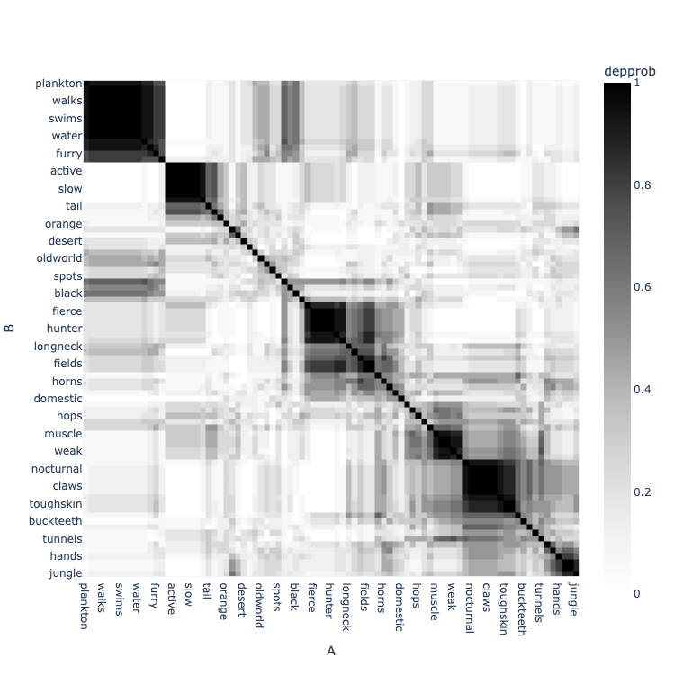
Above. A dependence probability clustermap. Each cell depresents the probability of dependence between two columns. Zero is white and black is one. The dendrogram, generated by seaborn, clusters mutual dependent columns.
It is important to note that dependence probability is meant to tell you whether a dependence exists; it does not necessarily provide information about the strength of dependencies. Dependence probability could potentially be high between independent columns if they are linked by dependent columns. For example, in the three-variable model
all three columns will be in the same view since Z is dependent on both X and Y, so there will be a high dependence probability between X and Y even though they are statistically independent, but they are dependent given Z.
Dependence probability is the go-to for structure modeling because it is fast to compute and well-behaved for all data. If you need more information about the strength of dependencies, use mutual information.
Mutual information
Mutual information (often referred to in code as mi) is a measure of the
information shared between two variables. Is is mathematically defined as
\[ I(X;Y) = \sum_{x \in X} \sum_{y \in Y} p(x,y) \log \frac{p(x, y)}{p(x)p(y)}, \]
or in terms of entropies,
\[ I(X;Y) = H(X) - H(X|Y). \]
Mutual information is well behaved for discrete data types (count and categorical), for which the sum applies; but for continuous data types for which the sum becomes an integral, mutual information can break down because differential entropy is no longer guaranteed to be positive.
For example, the following plots show the dependence probability and mutual information heatmaps for the zoo dataset, which is composed entirely of binary variables:
from lace import examples
animals = examples.Animals()
animals.clustermap('depprob', color_continuous_scale='greys', zmin=0, zmax=1)
Above. A dependence probability cluster map for the Animals dataset.
animals.clustermap('mi', color_continuous_scale='greys')
Above. A mutual information clustermap. Each cell represents the Mutual Information between two columns. Note that compared to dependence probability, the matrix is quite sparse. Also note that the diagonal entries are the entropies for each column.
And below are the dependence probability and mutual information heatmaps of the satellites dataset, which is composed of a mixture of categorical and continuous variables:
satellites = examples.Satellites()
satellites.clustermap('depprob', color_continuous_scale='greys', zmin=0, zmax=1)
Above. The dependence probability cluster map for the satellites date set.
satellites.clustermap('mi', color_continuous_scale='greys')
Above. The normalized mutual information cluster map for the satellites date set. Note that the values are no longer bounded between 0 and 1 due to inconsistencies caused by differential entropies.
satellites.clustermap(
'mi',
color_continuous_scale='greys',
fn_kwargs={'mi_type': 'linfoot'}
)
Above. The Linfoot-transformed mutual information cluster map for the satellites date set. The Linfoot information transformation often helps to mediate the weirdness that can arise from differential entropy.
Normalization Methods
Mutual information can be difficult to interpret because it does not have well-behaved bounds. In all but the continuous case (in which the mutual information could be negative), mutual information is only guaranteed to be greater than zero. To create an upper bound, we have a number of options:
Normalized
Knowing that the mutual information cannot exceed the minimum of the total information in (the entropy of) either X or Y, we can normalize by the minimum of the two component entropies:
\[ \hat{I}(X;Y) = \frac{I(X; Y)}{\min \left[H(X), H(Y) \right]} \]
animals.clustermap(
'mi',
color_continuous_scale='greys',
fn_kwargs={'mi_type': 'normed'}
)
Above. Normalized mutual information cluster map for the animals dataset.
IQR
In the Information Quality Ratio (IQR), we normalize by the joint entropy.
\[ \hat{I}(X;Y) = \frac{I(X; Y)}{H(X, Y)} \]
animals.clustermap(
'mi',
color_continuous_scale='greys',
fn_kwargs={'mi_type': 'iqr'}
)
Above. IQR Normalized mutual information cluster map for the animals dataset.
Jaccard
To compute the Jaccard distance, we subtract the IQR from 1. Thus, columns with more shared information have smaller distance
\[ \hat{I}(X;Y) = 1 - \frac{I(X; Y)}{H(X, Y)} \]
animals.clustermap(
'mi',
color_continuous_scale='greys',
fn_kwargs={'mi_type': 'jaccard'}
)
Above. Jaccard distance cluster map for the animals dataset.
Pearson
To compute something akin to the Pearson Correlation coefficient, we normalize by the square root of the product of the component entropies:
\[ \hat{I}(X;Y) = \frac{I(X; Y)}{\sqrt{H(X) H(Y)}} \]
animals.clustermap(
'mi',
color_continuous_scale='greys',
fn_kwargs={'mi_type': 'pearson'}
)
Above. Pearson normalized mutual information matrix cluster map for the animals dataset.
Linfoot
Linfoot information is the solution to solving for the correlation between the X and Y components of a bivariate Gaussian distribution with given mutual information.
\[ \hat{I}(X;Y) = \sqrt{ 1 - \exp(2 - I(X;Y)) } \]
animals.clustermap(
'mi',
color_continuous_scale='greys',
fn_kwargs={'mi_type': 'linfoot'}
)
Linfoot is often the most well-behaved normalization method especially when using continuous variables.
Above. Linfoot information matrix cluster map for the animals dataset.
Variation of Information
The Variation of Information (VOI) is a metric typically used to determine the distance between two clustering of variables, but we can use it generally to transform mutual information into a valid metric.
\[ \text{VI}(X;Y) = H(X) + H(Y) - 2 I(X,Y) \]
animals.clustermap(
'mi',
color_continuous_scale='greys',
fn_kwargs={'mi_type': 'voi'}
)
Above. Variation of information matrix.
Row similarity
Row similarity is (referred to in code as rowsim) a measurement of the similarity between rows. But row similarity is not a measurement of the distance between the values of the rows, but is a measure of how similarly the values of two rows are modeled. Row similarity is not a measurement in the data space, but in the model space. As such, we do not need to worry about coming up with an appropriate distance metric that incorporates data of different types, and we do not need to fret about missing data.
Rows whose values are modeled more similarly will have higher row similarity.
The technology underlying the Lace platform clusters columns into views, and within each view, clusters rows into categories. The row similarity is the average over states of the proportion of views in a state in which the two rows are in the same category.
\[ RS(A, B) \frac{1}{S} \sum_{s \in S} \frac{1}{V_s}\sum_{v \in V_s} [v_a = v_b] \]
Where S is the set of states, Vs is the set of assignments of rows in views to categories, and va is the assignment of row a in a particular view.
Column-weighted variant
One may wish to weight by the size of the view. For example, if 99% of the columns are in one view, and the two rows are together in the large view, but not the small view, we would like a row similarity of 99%, not 50%. For this reason, there is a column-weighted variant, which can be accessed by way of an extra argument to the rowsim function.
\[ \bar{RS}(A, B) \frac{1}{S} \sum_{s \in S} \sum_{v \in V_s} \frac{|C_v|}{|C|} [v_a = v_b] \]
where C is the set of all columns in the table and Cv is the number of columns in a given view, v.
We can see the effect of column weighting when computing the row similarity of animals in the zoo dataset.
from lace import examples
animals = examples.Animals()
animals.clustermap('rowsim', color_continuous_scale='greys', zmin=0, zmax=1)
Above. Standard row similarity for the animals data set.
animals.clustermap(
'rowsim',
color_continuous_scale='greys',
zmin=0,
zmax=1,
fn_kwargs={'col_weighted': True}
)
Above. Column-weighted row similarity for the animals data set. Note that the clusters are more pronounced.
Contextualization
Often, we are not interested in aggregate similarity over all variables, but in similarity with respect to specific target variables. For example, if we are an seeds company looking to determine where certain seeds will be more effective, we might not want to compute row similarity of locations across all variables, but might be more interested in row similarity with respect to yield.
Contextualized row similarity (usually via the wrt [with respect to] argument) is computed only over the views containing the columns of interest. When contextualizing with a single column, column-weighted and standard row similarity are equivalent.
animals.clustermap(
'rowsim',
color_continuous_scale='greys',
zmin=0,
zmax=1,
fn_kwargs={'wrt': ['swims']}
)
Above. Row similarity for the animals data set with respect to the swims variable. Animals that swim are colored blue. Animals that do not are colored tan. Note that if row similarity were looking at just the values of the data, similarity would either be zero (similar) or one (dissimilar) because the animals data are binary and we are looking it only one column. But row similarity here captures nuanced information about how swims is modeled. We see that withing the animals that swims, there are two distinct clusters of similarity. There are animals like the dolphin and killer whale that live their lives in the water, and there are animals like the polar bear and hippo that just visit. Both of these groups of animals swim, but for each group, Lace predicts that they swim for different reasons.
Likelihood
Computing likelihoods is the bread and butter of Lace. Apart from the clustering-based quantities, pretty much everything in Lace is computing likelihoods behind the scenes. Prediction is finding the argmax of a likelihood, surprisal is the negative likelihood, entropy is the integral of the production of the likelihood and log likelihood.
Computing likelihood is simple. First, we'll pull in the Satellites example.
import numpy as np
import pandas as pd
import plotly.graph_objects as go
from lace import examples
satellites = examples.Satellites()
We'll compute the univariate likelihood of the Period_minutes feature over a
range of values. We'll compute \(\log p(Period)\) and the conditional log
likelihood of period given that the satellite is geosynchronous, \( \log
p(Period | GEO)\).
period = pd.Series(np.linspace(0, 1500, 300), name="Period_minutes")
logp_period = satellites.logp(period)
logp_period_geo = satellites.logp(period, given={"Class_of_Orbit": "GEO"})
Rendered:
We can, of course compute likelihoods over multiple values:
values = pd.DataFrame({
'Period_minutes': [70.0, 320.0, 1440.0],
'Class_of_Orbit': ['LEO', 'MEO', 'GEO'],
})
values['logp'] = satellites.logp(values).exp()
values
Output (values):
| Class_of_Orbit | Period_minutes | logp | |
|---|---|---|---|
| 0 | LEO | 70 | 0.000364503 |
| 1 | MEO | 320 | 1.8201e-05 |
| 2 | GEO | 1440 | 0.0158273 |
We can find a close proximity to multivariate prediction by combining
simulate and logp.
# The things we observe
conditions = {
'Class_of_Orbit': 'LEO',
'Period_minutes': 80.0,
'Launch_Vehicle': 'Proton',
}
# Simulate many, many values
simulated = satellites.simulate(
['Country_of_Operator', 'Purpose', 'Expected_Lifetime'],
given=conditions,
n=100000, # big number
)
# compute the log likelihood of each draw given the conditions
logps = satellites.logp(simulated, given=conditions)
# return the draw with the highest likelihood
simulated[logps.arg_max()]
Output:
shape: (1, 3)
┌─────────────────────┬────────────────┬───────────────────┐
│ Country_of_Operator ┆ Purpose ┆ Expected_Lifetime │
│ --- ┆ --- ┆ --- │
│ str ┆ str ┆ f64 │
╞═════════════════════╪════════════════╪═══════════════════╡
│ USA ┆ Communications ┆ 7.554264 │
└─────────────────────┴────────────────┴───────────────────┘
Prediction & Imputation
Prediction and imputation both involve inferring an unknown quantity. Imputation refers to inferring the value of a specific cell in our table, and prediction refers to inferring a hypothetical value.
The arguments for impute are the coordinates of the cell. We may wish to impute the cell at row bat and column furry. The arguments for prediction are the conditions we would like to use to create the conditional distribution. We may wish to predict furry given flys=True, brown=True, and fierce=False.
Uncertainty
Uncertainty comes from several sources (to learn more about those sources, check out this blog post):
- Natural noise/imprecision/variance in the data-generating process
- Missing data and features
- Difficulty on the part of the model to capture a prediction
Type 1 uncertainty can be captured by computing the predictive distribution variance (or entropy for categorical targets). You can also visualize the predictive distribution. Observing multi-modality (multiple peaks in the distribution) can be a good indication that you are missing valuable information.
Determining how certain the model is in its ability to capture a prediction is done by assessing the consensus among the predictive distribution emitted by each state. The more alike these distributions are, the more certain the model is in its ability to capture a prediction.
Mathematically, uncertainty is formalized as the Jensen-Shannon divergence (JSD) between the state-level predictive distributions. Uncertainty goes from 0 to 1, 0 meaning that there is only one way to model a prediction, and 1 meaning that there are many ways to model a prediction and they all completely disagree.
import pandas as pd
from lace import examples, plot
satellites = examples.Satellites()
plot.prediction_uncertainty(
satellites,
"Period_minutes",
given={ "Class_of_Orbit": "GEO"}
)
Above. Prediction uncertainty when predicting Period_minutes of a geosynchronous satellite in the satellites dataset. Uncertainty is low. Though the stat distributions differ slightly in their variance, they're relatively close, with similar means.
To visualize a higher uncertainty prediction, well use given conditions from a record with a know data entry error.
given = satellites["Intelsat 902", :].to_dicts()[0]
# remove all missing data
given = { k: v for k, v in given.items() if not pd.isnull(v) }
# remove the index and the target value
_ = given.pop("index")
_ = given.pop("Period_minutes")
plot.prediction_uncertainty(
satellites,
"Period_minutes",
given=given
)
Above. Prediction uncertainty when predicting Period_minutes of Intelsat 902. Though the mean predictive distribution (black line) has a relatively low variance, there is a lot of disagreement between some of the samples, leading to high epistemic uncertainty.
Certain ignorance is when the model has zero data by which to make a prediction and instead falls back to the prior distribution. This is rare, but when it happens it will be apparent. To be as general as possible, the priors for a column's component distributions are generally much more broad than the predictive distribution, so if you see a predictive distribution that is senselessly wide and does not looks like the marginal distribution of that variable (which should follow the histogram of the data), you have a certain ignorance. The fix is to fill in the data for items similar to the one you are predicting.
Surprisal
Surprisal is a method by which users may find surprising (go figure) data such as outliers, anomalies, and errors.
In information theory
In information theoretic terms, "surprisal" (also referred to as self-information, information content, and potentially other things) is simply the negative log likelihood.
\[ s(x) = -\log p(x) \ \]
\[ s(x|y) = -\log p(x|y) \]
In Lace
In the Lace Engine, you have the option to call engine.surprisal and the option
the call -engine.logp. There are differences between these two calls:
engine.surprisal takes a column as the first argument and can take optional row
indices and values. engine.surprisal computes the information theoretic surprisal
of a value in a particular position in the Lace table. engine.surprisal considers
only existing values, or hypothetical values at specific positions in the
table.
-engine.logp considers hypothetical values only. We provide a set of inputs and
conditions and as 'how surprised would we be if we saw this?'
As an example, we can ask lace for the top 10 most surprisingly fierce animals
from the Animals dataset.
from lace.examples import Animals
animals = Animals()
animals.surprisal("fierce")\
.sort("surprisal", descending=True)\
.head(10)
Output:
# polars
shape: (10, 3)
┌──────────────┬────────┬───────────┐
│ index ┆ fierce ┆ surprisal │
│ --- ┆ --- ┆ --- │
│ str ┆ u32 ┆ f64 │
╞══════════════╪════════╪═══════════╡
│ pig ┆ 1 ┆ 1.565845 │
│ rhinoceros ┆ 1 ┆ 1.094639 │
│ buffalo ┆ 1 ┆ 1.094639 │
│ chihuahua ┆ 1 ┆ 0.802085 │
│ ... ┆ ... ┆ ... │
│ collie ┆ 0 ┆ 0.594919 │
│ otter ┆ 0 ┆ 0.386639 │
│ hippopotamus ┆ 0 ┆ 0.328759 │
│ persian+cat ┆ 0 ┆ 0.322771 │
└──────────────┴────────┴───────────┘
Interpreting surprisal values
Surprisal is not normalized insofar as the likelihood is not normalized. For discrete distributions, surprisal will always be positive, but for tight continuous distributions that can have likelihoods greater than 1, surprisal can be negative. Interpreting the raw surprisal values is simply a matter of looking at which values are higher or lower and by how much.
Transformations may not be very useful. The surprised distribution is usually very far from capital 'N' Normal (Gaussian).
import plotly.express as px
from lace.examples import Satellites
engine = Satellites()
surp = engine.surprisal('Period_minutes')
# plotly support for polars isn't currently great
fig = px.histogram(surp.to_pandas(), x='surprisal')
fig.show()
Lots of skew in this distribution. The satellites example is especially nasty because there are a lot of extremes when we're talking about spacecraft.
Simulating data
If you've used logp, you already understand how to simulate data. In both
logp and simulate you define a distribution. In logp the output is an
evaluation of a specific point (or points) in the distribution; in simulate
you generate from the distribution.
We can simulate from joint distributions
from lace.examples import Animals
animals = Animals()
swims = animals.simulate(['swims'], n=10)
Output:
shape: (10, 1)
┌───────┐
│ swims │
│ --- │
│ u32 │
╞═══════╡
│ 1 │
│ 0 │
│ 0 │
│ 0 │
│ ... │
│ 0 │
│ 0 │
│ 0 │
│ 0 │
└───────┘
Or we can simulate from conditional distributions
swims = animals.simulate(['swims'], given={'flippers': 1}, n=10)
Output:
shape: (10, 1)
┌───────┐
│ swims │
│ --- │
│ u32 │
╞═══════╡
│ 1 │
│ 1 │
│ 1 │
│ 1 │
│ ... │
│ 1 │
│ 0 │
│ 1 │
│ 0 │
└───────┘
We can simulate multiple values
animals.simulate(
['swims', 'coastal', 'furry'],
given={'flippers': 1},
n=10
)
Output:
shape: (10, 3)
┌───────┬─────────┬───────┐
│ swims ┆ coastal ┆ furry │
│ --- ┆ --- ┆ --- │
│ u32 ┆ u32 ┆ u32 │
╞═══════╪═════════╪═══════╡
│ 1 ┆ 1 ┆ 0 │
│ 0 ┆ 0 ┆ 1 │
│ 1 ┆ 1 ┆ 0 │
│ 1 ┆ 1 ┆ 0 │
│ ... ┆ ... ┆ ... │
│ 1 ┆ 1 ┆ 0 │
│ 1 ┆ 1 ┆ 0 │
│ 1 ┆ 1 ┆ 1 │
│ 1 ┆ 1 ┆ 1 │
└───────┴─────────┴───────┘
If we want to create a debiased dataset we can do something like this: There are too many land animals in the animals dataset, we'd like an even representation of land and aquatic animals. All we need to do is simulate from the conditionals and concatenate the results.
import polars as pl
n = animals.n_rows
target_col = 'swims'
other_cols = [col for col in animals.columns if col != target_col]
land_animals = animals.simulate(
other_cols,
given={target_col: 0},
n=n//2,
include_given=True
)
aquatic_animals = animals.simulate(
other_cols,
given={target_col: 1},
n=n//2,
include_given=True
)
df = pl.concat([land_animals, aquatic_animals])
Output:
# polars df
shape: (50, 85)
┌───────┬───────┬──────┬───────┬─────┬──────────┬──────────┬──────────┬───────┐
│ black ┆ white ┆ blue ┆ brown ┆ ... ┆ solitary ┆ nestspot ┆ domestic ┆ swims │
│ --- ┆ --- ┆ --- ┆ --- ┆ ┆ --- ┆ --- ┆ --- ┆ --- │
│ u32 ┆ u32 ┆ u32 ┆ u32 ┆ ┆ u32 ┆ u32 ┆ u32 ┆ i64 │
╞═══════╪═══════╪══════╪═══════╪═════╪══════════╪══════════╪══════════╪═══════╡
│ 1 ┆ 0 ┆ 0 ┆ 1 ┆ ... ┆ 0 ┆ 0 ┆ 0 ┆ 0 │
│ 1 ┆ 0 ┆ 0 ┆ 1 ┆ ... ┆ 1 ┆ 1 ┆ 0 ┆ 0 │
│ 1 ┆ 0 ┆ 0 ┆ 1 ┆ ... ┆ 0 ┆ 0 ┆ 0 ┆ 0 │
│ 0 ┆ 1 ┆ 0 ┆ 0 ┆ ... ┆ 0 ┆ 0 ┆ 0 ┆ 0 │
│ ... ┆ ... ┆ ... ┆ ... ┆ ... ┆ ... ┆ ... ┆ ... ┆ ... │
│ 1 ┆ 1 ┆ 0 ┆ 1 ┆ ... ┆ 0 ┆ 1 ┆ 1 ┆ 1 │
│ 1 ┆ 1 ┆ 0 ┆ 1 ┆ ... ┆ 1 ┆ 0 ┆ 0 ┆ 1 │
│ 1 ┆ 1 ┆ 0 ┆ 1 ┆ ... ┆ 0 ┆ 0 ┆ 0 ┆ 1 │
│ 0 ┆ 0 ┆ 0 ┆ 0 ┆ ... ┆ 0 ┆ 0 ┆ 1 ┆ 1 │
└───────┴───────┴──────┴───────┴─────┴──────────┴──────────┴──────────┴───────┘
That's it! We introduced a new keyword argument, include_given, which
includes the given conditions in the output so we don't have to add them back
manually.
The draw method
The draw method is the in-table version of simulate. draw takes the row
and column indices and produces values from the probability distribution
describing that specific cell in the table.
otter_swims = animals.draw('otter', 'swims', n=5)
Output:
shape: (5,)
Series: 'swims' [u32]
[
1
1
1
1
1
]
Evaluating simulated data
There are a number of ways to evaluate the quality of simulated (synthetic) data:
- Overlay histograms of synthetic data over histograms of the real data for each variable.
- Compare the correlation matrices emitted by the real and synthetic data.
- Train a classifier to classify real and synthetic data. The better the synthetic data, the more difficult it will be for a classifier to identify synthetic data. Note that you must consider the precision of the data. Lace simulates full precision data. If the real data are rounded to a smaller number of decimal places, a classifier may pick up on that. To fix this, simply round the simulated data.
- Train a model on synthetic data and compare its performance on a real-data test set against a model trained on real data. Close performance to the real-data-trained model indicates higher quality synthetic data.
If you are concerned about sensitive information leakage, you should also measure the similarity each synthetic record to each real record. Secure synthetic data should not contain records that are so so to the originals that they may reproduce sensitive information.
In- and out-of-table operations
In Lace there are a number of operations that seem redundant. Why is there
simulate and draw; predict and impute? Why is there surprisal when
one can simple compute -logp? The answer is that the are in-table operations
and out-of-table (or hypothetical) operations. In-table operations use the
probability distribution at a certain cell in the PCC table, while out-of-table
operations do not take table location, and thus category and view assignments
into account. Hypothetical operations must marginalize over assignments.
Here is a table listing in-table and hypothetical operations.
| Purpose | In-table | Hypothetical |
|---|---|---|
| Draw random data | draw | simulate |
| Compute likelihood | (-) surprisal | logp |
| Find argmax of a likelihood | impute | predict |
Adding data to a model
Lace allow you to add and edit data without having to completely re-train.
You can edit existing cells,
import pandas as pd
from lace.examples import Animals
animals = Animals()
animals.edit_cell(row='pig', col='fierce', value=0)
assert animals['pig', 'fierce'] == 0
use lace::examples::Example;
use lace::prelude::*;
let mut animals = Example::Animals.engine().unwrap();
let write_mode = WriteMode::unrestricted();
let rows = vec![Row {
row_ix: String::from("pig"),
values: vec![Value {
col_ix: String::from("fierce"),
value: Datum::Categorical(lace::Category::UInt(0)),
}],
}];
animals.insert_data(rows, None, write_mode).unwrap();you can remove existing cells (set the value as missing),
animals.edit_cell(row='otter', col='brown', value=None)
assert animals['otter', 'brown'] is None
let write_mode = WriteMode::unrestricted();
let rows = vec![Row {
row_ix: String::from("otter"),
values: vec![Value {
col_ix: String::from("spots"),
value: Datum::Missing,
}],
}];
animals.insert_data(rows, None, write_mode).unwrap();you can append new rows,
animals.append_rows({
'tribble': {'fierce': 1, 'meatteeth': 0, 'furry': 1},
})
assert animals['tribble', 'fierce'] == 1
let write_mode = WriteMode::unrestricted();
let tribble = vec![Row {
row_ix: String::from("tribble"),
values: vec![
Value {
col_ix: String::from("fierce"),
value: Datum::Categorical(lace::Category::UInt(1)),
},
Value {
col_ix: String::from("meatteeth"),
value: Datum::Categorical(lace::Category::UInt(0)),
},
Value {
col_ix: String::from("furry"),
value: Datum::Categorical(lace::Category::UInt(1)),
},
],
}];
animals.insert_data(tribble, None, write_mode).unwrap();and you can even append new columns.
cols = pd.DataFrame(
pd.Series(["blue", "geen", "blue", "red"], name="fav_color", index=["otter", "giant+panda", "dolphin", "bat"])
)
# lace will infer the column metadata, or you can pass the metadata in
animals.append_columns(cols)
assert animals["bat", "fav_color"] == "red"
Some times you may need to supply lace with metadata about the column.
from lace import ColumnMetadata, ContinuousPrior
cols = pd.DataFrame(
pd.Series([0.0, 0.1, 2.1, -1.3], name="fav_real_number", index=["otter", "giant+panda", "dolphin", "bat"])
)
md = ColumnMetadata.continuous(
"fav_real_number",
prior=ContinuousPrior(0.0, 1.0, 1.0, 1.0)
)
animals.append_columns(cols, metadata=[md])
assert animals["otter", "fav_real_number"] == 0.0
assert animals["antelope", "fav_real_number"] is None
Note that when you add a column you'll need to run inference (fit) a bit to incorporate the new information.
Prior Processes
In Lace (and in Bayesian nonparametrics) we put a prior on the number of parameters. This prior process formalizes how instances are distributed to an unknown number of categories. Lace gives you two options
- The one-parameter Dirichlet process,
DP(α) - The two-parameter Pitman-Yor process,
PYP(α, d)
The Dirichlet process more heavily penalizes new categories with an exponential fall off while the Pitman-Yor process has a power law fall off in the number for categories. When d = 0, Pitman-Yor is equivalent to the Dirichlet process.
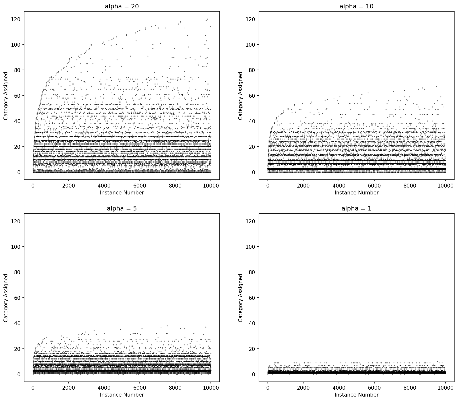
Figure: Category ID (y-axis) by instance number (x-axis) for Dirichlet process draws for various values of alpha.
Pitman-Yor may fit the data better but (and because) it will create more parameters, which will cause model training to take longer.
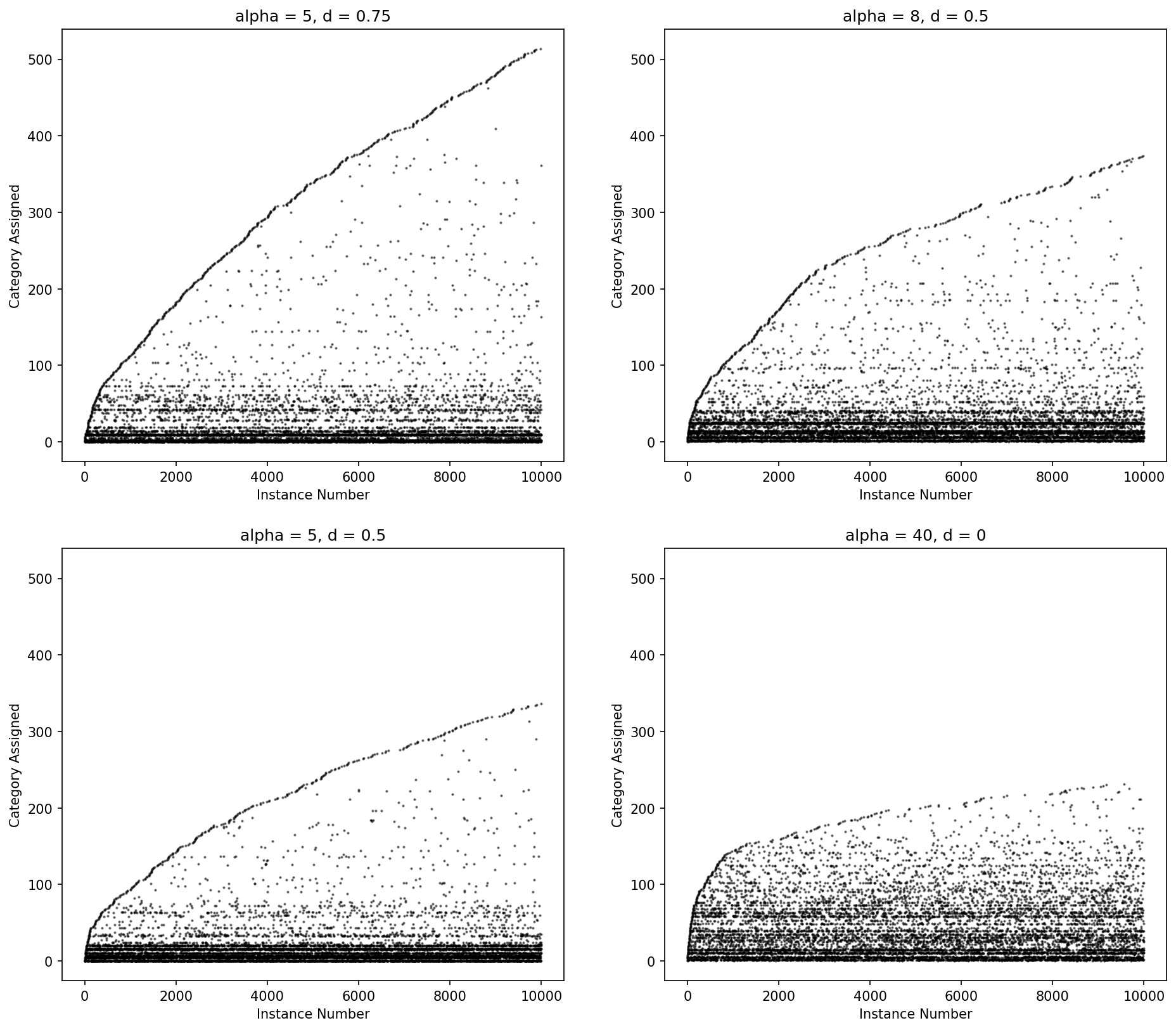
Figure: Category ID (y-axis) by instance number (x-axis) for Pitman-Yor process draws for various values of alpha and d.
For those looking for a good introduction to prior process, this slide deck from Yee Whye Teh is a good resource.
Preparing your data for Lace
Compared with many other machine learning tools, lace has very few requirements
for data: data columns may be integer, continuous, or categorical string types;
empty cells do not not need to be filled in; and the table must contain a
string row index column labeled ID or Index (case-insensitive).
Supported data types for inference
Lace supports several data types, and more can be supported (with some work from us).
Continuous data
Continuous columns are modeled as mixtures of Gaussian distributions. Find an explanation of the parameters in the codebook
Categorical data
Categorical columns are modeled as mixtures of categorical distributions. Find an explanation of the parameters in the codebook.
Count data
Support exists for a count data type, which is modeled as a mixture of Poission distributions, but there are some drawbacks, which make it best to convert the data to continuous in most cases.
- The Poisson distribution is a single parameter model so the location and variance of the mixture components cannot be controlled individually. In the Poisson model, higher magnitude means higher variance.
- The hyper prior for count data is finicky and can often cause underflow/overflow errors when the underlying data do not look like Poisson distributions.
Note: If you use Count data, do so because you know that the underlying mixture components will be Poisson-like and be sure to set the prior and unset the hyperprior in the codebook
Preparing your data for Lace
Lace is pretty forgiving when it comes to data. You can have missing values, string values, and numerical values all in the same table; but there are some rules that your data must follow for the platform to pick up on things. Here you will learn how to make sure Lace understands your data properly.
Accepted formats
Lace currently accepts the following data formats
- CSV
- CSV.gz (gzipped CSV)
- Parquet
- IPC (Apache Arrow v2)
- JSON (as output by the pandas function
df.to_json('mydata.json)) - JSON Lines
Using a schemaless data format
Formatting your data properly will help the platform understand your data.
Under the hood, Lace uses polars for reading data formats into a DataFrame.
For more information about i/o in polars, see the polars API
documentation.
Here are the rules:
- Real-valued (continuous data) cells must have decimals.
- Integer-valued cells, whether count or categorical, must not have decimals.
- Categorical data cells may be integers (up to 255) or string values
- In a CSV, missing cells should be empty
- A row index is required. The index label should be 'ID'.
Not following these rules will confuse the codebook and could cause parsing errors.
Row and column names
Row and column indices or names must be strings. If you were to create a codebook from a csv with integer row and column indices, Lace would convert them to strings.
Tips on creating valid data with pandas
When reading data from a CSV, Pandas will convert integer columns with missing
cells to float values since floats can represent NaN, which is how pandas
represents missing data. You have a couple of options for saving your CSV file
with both missing cells and properly formatted integers:
You can coerce the types to Int64, which is basically Int plus NaN, and
then write to CSV.
import pandas as pd
df = pd.DataFrame([10,20,30], columns=['my_int_col'])
df['my_int_col'] = df['my_int_col'].astype('Int64')
df.to_csv('mydata.csv', index_label='ID')
If you have a lot of columns or particularly long columns, you might find it
much faster just to reformat as you write to the csv, in which case you can
use the float_format option in DataFrame.to_csv
df.to_csv('mydata.csv', index_label='ID', float_format='%g')
Codebook reference
The codebook is how you tell Lace about your data. The codebook contains information about
- Row names
- Column names
- The type of data in each column (e.g., continuous, categorical, or count)
- The prior on the parameters for each column
- The hyperprior on the prior parameters for each column
- The prior on the Dirichlet Process alpha parameter
Codebook fields
table_name
String name of the table. For your reference.
state_prior_process
The prior process used for assigning columns to views. Can either be a Dirichlet process with a Gamma prior on alpha:
state_prior_process: !dirichlet
alpha_prior:
shape: 1.0
rate: 1.0
or a Pitman-Yor process with a Gamma prior on alpha and a Beta prior on d.
state_prior_process: !pitman_yor
alpha_prior:
shape: 1.0
rate: 1.0
d_prior:
alpha: 0.5
beta: 0.5
view_prior_process
The prior process used for assigning rows to categories. Can either be a Dirichlet process with a Gamma prior on alpha:
view_prior_process: !dirichlet
alpha_prior:
shape: 1.0
rate: 1.0
or a Pitman-Yor process with a Gamma prior on alpha and a Beta prior on d.
view_prior_process: !pitman_yor
alpha_prior:
shape: 1.0
rate: 1.0
d_prior:
alpha: 0.5
beta: 0.5
col_metadata
A list of columns, ordered by left-to-right occurrence in the data. Contains the following fields:
name: The name of the columnnotes: Optional information about the column. Purely for referencecoltype: Contains information about the type type of data, the prior, and the hyper prior. See column metadata for more informationmissing_not_at_random: a boolean. Iffalse(default), missing values in the column are assumed to be missing completely at random.
row_names
A list of row names in order of top-to-bottom occurrence in the data
notes
Optional notes for user reference
Codebook type inference
When you upload your data, Lace will pull the row and column names from the file, infer the data types, and choose and empirical hyperprior from the data.
Type inference works like this:
- Categorical if:
- The column contains only string values
- Lace will assume the categorical variable can take on any of (and only) the existing values in the column
- There are only integers up to a cutoff.
- If There are only integers in the column
xthe categorical values will be assumed to take on values 0 tomax(x).
- If There are only integers in the column
- The column contains only string values
- Count if:
- There are only integers that exceed the value of the cutoff
- Continuous if:
- There are only integers and one or more floats
Column metadata
- Either
priororhypermust be defined.- If
prioris defined andhyperis not defined, hyperpriors and hyperparameter inference will be disabled.
- If
It is best to leave the hyperpriors alone. It is difficult to intuit what effect the hyperpriors have on the final distribution. If you have knowledge beyond the vague hyperpriors, null out the `hyper` field with a `~` and set the prior instead. This will disable hyperparameter inference inf favor of the expert knowledge you have provided.
Continuous
The continuous type has the hyper field and the prior field. The prior
parameters are those for the Normal Inverse Chi-squared prior on the mean and
variance of a normal distribution.
m: the prior meank: how strongly (in pseudo observations) that we believems2: the prior variancev: how strongly (is pseudo observations) that we believes2
To have widely dispersed components with small variances you would set k very
low and very high.
FIXME: Animation showing effect of different priors
The hyper priors are the priors on the above parameters. They are named for the
parameters to which they are attached, e.g. pr_m is the hyper prior for the
m parameter.
pr_m: Normal distributionpr_k: Gamma distribution with shape and rate (inverse scale) parameterspr_v: Inverse gamma distribution with shape and scale parameterspr_s2: Inverse gamma distribution with shape and scale parameters
- name: Eccentricity
coltype: !Continuous
hyper:
pr_m:
mu: 0.02465318142734303
sigma: 0.1262297091840037
pr_k:
shape: 1.0
rate: 1.0
pr_v:
shape: 7.0587581525186648
scale: 7.0587581525186648
pr_s2:
shape: 7.0587581525186648
scale: 0.015933939480678149
prior:
m: 0.0
k: 1.0
s2: 7.0
v: 1.0
# To not define the prior add a `~`
# prior: ~
notes: ~
missing_not_at_random: false
Categorical
In addition to prior and hyper, Categorical has additional special fields:
k: the number of values the variable can assumevalue_map: An optional map of integers in [0, ..., k-1] mapping the integer code (how the value is represented internally) to the string value. Ifvalue_mapis not defined, it is usually assume that classes take on only integer values in [0, ..., k-1].
The hyper is an inverse gamma prior on the prior parameter alpha
- name: Class_of_Orbit
coltype: !Categorical
k: 4
hyper:
pr_alpha:
shape: 1.0
scale: 1.0
value_map: !string
0: Elliptical
1: GEO
2: LEO
3: MEO
prior:
alpha: 0.5
k: 4
# To not define the prior add a `~`
# prior: ~
notes: ~
missing_not_at_random: false
Editing the codebook
You should use the default codebook generated by the Lace CLI as a starting point for custom edits. Generally the only edits you will make are
- Adding notes/comments
- changing the
state_alpha_priorandview_alpha_prior(though you should only do this if you know what you're doing) - converting a
Countcolumn to aCategoricalcolumn. Usually there will be no need to change between other column types.
Appendix
Stats primer
What you need to know about Bayesian Statistics
Bayesian statistics is built around the idea of posterior inference. The posterior distribution is the probability distribution of the parameters, \(\theta\), of some model given observed data, \(x\). In math: \( p(\theta | s) \). Per Bayes theorem, the posterior distribution can be written in terms of other distributions,
\[ p(\theta | s) = \frac{p(x|\theta)p(\theta)}{p(x)}. \]
Where \( p(x|\theta) \) is the likelihood of the observations given the parameters of our model; \( p(\theta) \) is the prior distribution, which defines our beliefs about the model parameters in the absence of data; and \( p(x) \) is the marginal likelihood, which the likelihood of the data marginalized over all possible models. Of these, the likelihood and prior are the two distributions we're most concerned with. The marginal likelihood, which is defined as
\[ p(x) = \int p(x|\theta)p(\theta) d\theta \]
is notoriously difficult and a lot of effort in Bayesian computation goes toward making the marginal likelihood go away, so we won't talk about it much.
Finite mixture models
A mixture model is a weighted sum of probabilistic distributions. Here is an example of bimodal mixture model.
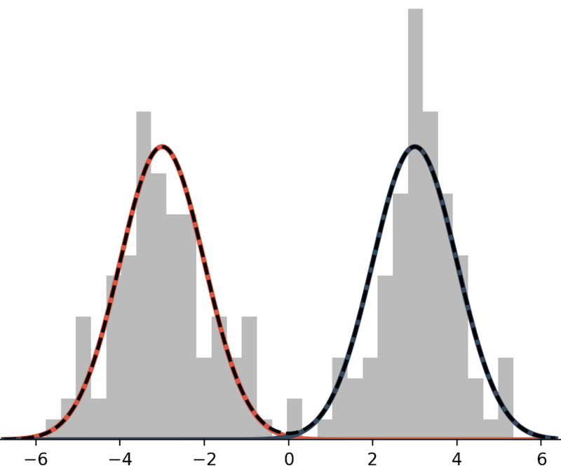
This mixture model is defined as the sum of two Normal distributions:
\[ p(x) = \frac{1}{2} N(x; \mu=-3, \sigma^2=1) + \frac{1}{2} N(x; \mu=3, \sigma^2=1). \]
In lace, we will often use the term mixture component to refer to an individual model within a mixture.
In general a mixture distribution has the form
\[ p(x|\theta) = \sum_{i=1}^K w_i , p(x|\theta_i), \]
where \(K\) is the number of mixture components, \(w_i\) is the \(i^{th}\) weight, and all weights are positive and sum to 1.
To draw a mixture model from the prior,
- Draw the weights, \( w \sim \text{Dirichlet}(\alpha) \), where \(\alpha\) is a \(K\)-length vector of values in \((0, \infty)\).
- For \(i \in {1, ..., K}\) draw \( \theta_i \sim p(\theta) \)
As a note, we usually use one \(\alpha\) value repeated \(K\) times rather than \(K\) distinct values. We do not often have reason to think that any one component is more likely than the other, and reducing a vector to one value reduces the number of dimensions in our model.
Dirichlet process mixture models (DPMM)
Suppose we don't know how many components are in our model. Given \(N\) data, there could be as few as 1 and as many as \(N\) components. To infer the number of components or categories, we place a prior on how categories are formed. One such prior is the Dirichlet process. To explain the Dirichlet process we use the Chinese restaurant process (CRP) formalization.
The CRP metaphor works like this: you are on your lunch break and, as one often does, you to usual luncheon spot: a magical Chinese restaurant where the rules of reality do not apply. Today you happen to arrive a bit before open and, as such, are the first customer to be seated. There is exactly one table with exactly one seat. You sit at that table. Or was the table instantiated for you? Who knows. The next customer arrives. They have a choice. They can sit with you or they can sit at a table alone. Customers at this restaurant love to sit together (customers of interdimensional restaurants tend to be very social creatures), but the owners offer a discount to customers who instantiate new tables. Mathematically, a customer sits at a table with probability
\[ p(z_i = k) = \begin{cases} \frac{n_k}{N_{-i}+\alpha}, & \text{if $k$ exists} \\ \frac{\alpha}{N_{-i}+\alpha}, & \text{otherwise} \end{cases}, \]
where \(z_i\) is the table of customer i, \(n_k\) is the number of customers currently seated at table \(k\), and \(N_{-i}\) is the total number of seated customers, not including customer i (who is still deciding where to sit).
Under the CRP formalism, we make inferences about what datum belongs to which category. The weight vector is implicit. That's it. For information on how inference is done in DPMMs check out the literature recommendations.
Glossary
Here we list some of the terminology, including acronyms, you will encounter when using lace.
- view: A cluster of columns within a state.
- category: A cluster of rows within a view.
- component model: The probability distribution defining the model of a specific category in a column.
- state: what we call a lace posterior sample. Each state represents the current configuration (or state) of an independent markov chain. We aggregate over states to achieve estimate of likelihoods and uncertainties.
- metadata: A set of files from which an
Enginemay be loaded - prior: A probability distribution that describe how likely certain hypotheses (model parameters) are before we observe any data.
- hyperprior: A prior distribution on prior. Allows us to admit a larger amount of initial uncertainty and permit a broader set of hypotheses.
- empirical hyperprior: A hyperprior with parameters derived from data.
- CRP: Chinese restaurant process
- DPMM: Dirichlet process mixture model
- PCC: Probabilistic cross-categorization
References
Bayesian statistics and information theory
For an introduction to Bayesian statistics, information theory, and Markov chain Monte Carlo (MCMC), David MacKay's "Information Theory, Inference and Learning Algorithms" 1 is an excellent choice and it's available for free.
Dirichlet process mixture models
For an introduction to infinite mixture models via the Dirichlet process, Carl Rasumssen's "The infinite Gaussian mixture model"2 provides an introduction to the model; and Radford Neal's "Markov chain sampling methods for Dirichlet process mixture models"3 provides an introduction to basic MCMC methods. When I was learning Dirichlet process mixture models, I found Frank Wood and Michael Black's "A nonparametric Bayesian alternative to spike sorting" 4 extremely helpful. Because its target audience is applied scientists it lays things out more simply and completely than a manuscript aimed at statisticians or computer scientists might.
Probabilistic cross-categorization (PCC)
For a compact explanation designed for people unfamiliar with Bayesian statistics, see Shafto, et al 5. This work is targeted at psychologists and demonstrates PCC's power to model human cognitive capabilities. For a incredibly in-dept overview with loads of math, use cases, and examples, see Mansinghka et al 6.
-
MacKay, D. J., & Mac Kay, D. J. (2003). Information theory, inference and learning algorithms. Cambridge university press. (PDF) ↩
-
Rasmussen, C. (1999). The infinite Gaussian mixture model. Advances in neural information processing systems, 12. (PDF) ↩
-
Neal, R. M. (2000). Markov chain sampling methods for Dirichlet process mixture models. Journal of computational and graphical statistics, 9(2), 249-265. (PDF) ↩
-
Wood, F., & Black, M. J. (2008). A nonparametric Bayesian alternative to spike sorting. Journal of neuroscience methods, 173(1), 1-12. (PDF) ↩
-
Shafto, P., Kemp, C., Mansinghka, V., & Tenenbaum, J. B. (2011). A probabilistic model of cross-categorization. Cognition, 120(1), 1-25.(PDF) ↩
-
Mansinghka, V., Shafto, P., Jonas, E., Petschulat, C., Gasner, M., & Tenenbaum, J. B. (2016). Crosscat: A fully bayesian nonparametric method for analyzing heterogeneous, high dimensional data. (PDF) ↩